2.70 Precision Machine Design Spring 2019
In this class, we are to make a new device biweekly to demonstrate a particular fundametal theory of design. These devices are called FPGA - FUNdaMENTAL Principle Gizmo Assignments. The goal is to do the math to predict its performance and then build it. Along with my partner, Chetan Sharma, we created six FPGAs in this class.
FPGA 1: Preload
Finicky Preload with Great Applications
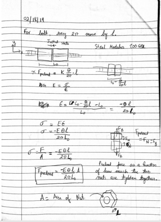
In this week FPGA, we wanted to demonstrate how you can create a locknut by using two nuts. This is accomplished by taking two nuts and tightening (preloading) it together.
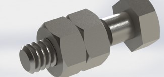
We wanted to see how much torque this artificial locknut can resist. We created an analytical model to predict its performance.
 |
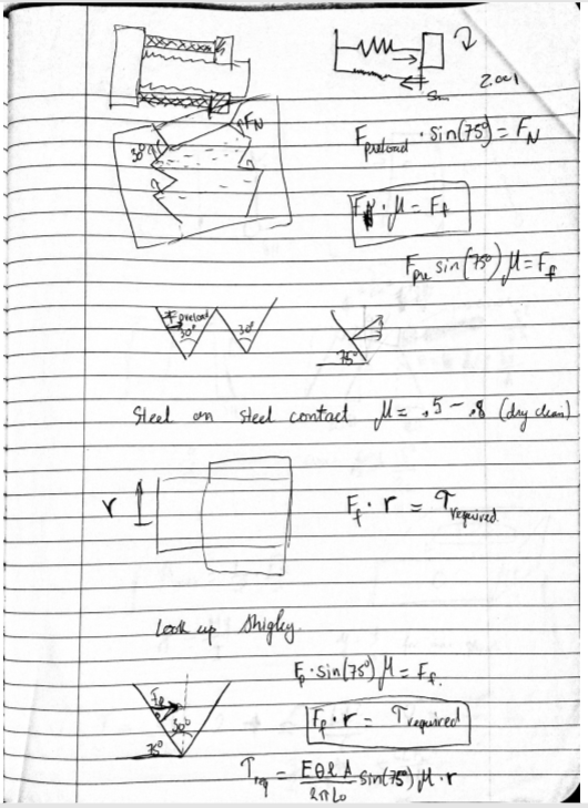 |
We then created a matlab script to do this calculation for us.
(click to see code)
%% FPGA 1

%% parameters
E = 200 * 10^9; %steel 200 GPa
l = 1/20 * 0.0254; %lead = 1/20 in
L = 7/32*2 * 0.0254; %length of assemble (m)
u = 0.5; % coefficient of friction
r = 1/8 * 0.0254; %radius of bolt

%% derived parameters
A = (((7/16)/2)^2 *pi - ((1/4)/2)^2 *pi) * 0.0254^2; % m^2 front area of nut

%% Do calculation
f1 = @computeForce;
f2 = @computeTorque;

%% Function
% Put in equations form
function force = computeForce(original, final)
    A = (((7/16)/2)^2 *pi - ((1/4)/2)^2 *pi) * 0.0254^2; % m^2 front area of nut
    strain = ((final - original)/original)/2;
    E = 190 * 10^9;
    stress = strain*E;
    force = stress * A;
end
function torque = computeTorque(preload)
    u = 0.5;
    r = 1/8 * 0.0254;
    torque = preload*sind(75)*u*r;
end
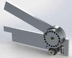
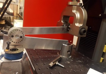
The actual device that we built is a jig that hold the two preloaded nuts together, so we can test it resistance to torque with a mini Instron machine.
 |
 |
Our mathematical model could predict the preloaded nut if we use a spring washer in between the buts. However, if we just smash two nuts together, the mechanic becomes more complicated as we have to account for the uneven tensioning of the threads.
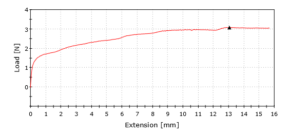
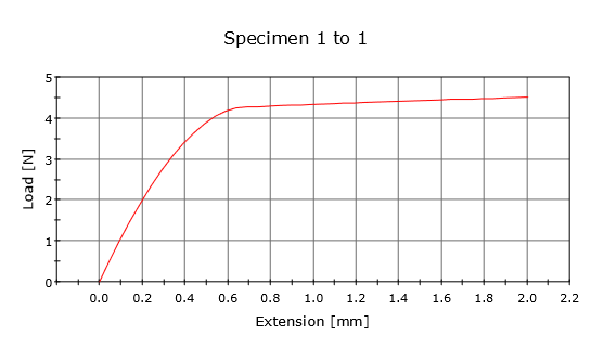
Trial 1 (Spring Washer 180 deg) Preload = 152.4 N Finput predict = 2.33 N Finput actual = 3 N
Trial 2 (Spring Washer 360 deg) Preload = 304.8 N Finput predict = 4.67 N Finput actual = 4.5 N
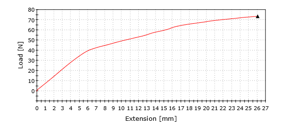
Trial 3 (Smashing Nuts 10 deg) Preload = 19699 N Finput predict = 151.1 N Finput actual = 72 N
FPGA 2: St. Venant, Golden Rectangle, Stability
Figure Pondering Grading of Assignment
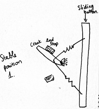
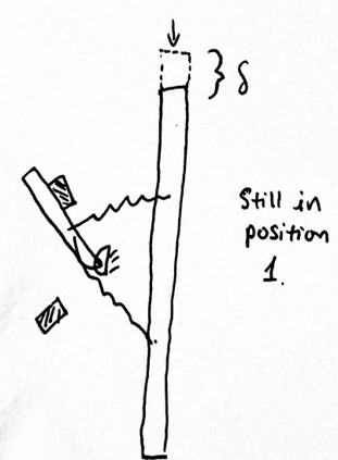
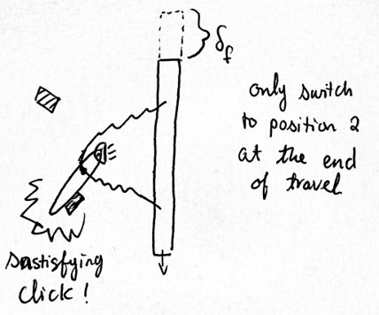
In this FPGA, we wanted to create the most satisfying switch possible. The semi-bistable switch we created demonstrate the fundamental design of stability.
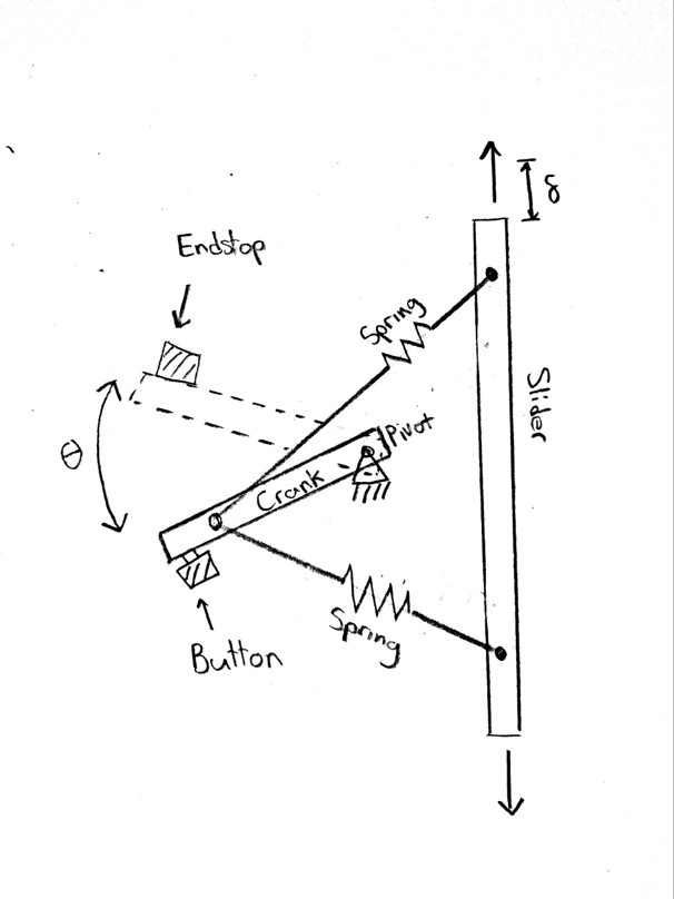
In order to create the clicking sound, we made an elastic system with hysteresis. The crank is stable in one position during the full travel of the button and only changes to another stable position at the end of the button’s travel.
 |
 |
 |
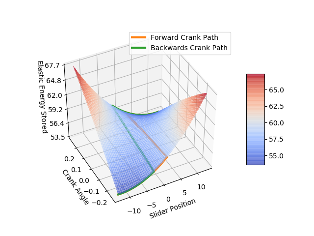
This behavior is calculated using a python script. The script describe the energy stored in system as the button is being pressed. As the system has hysterisis, it will switch from one state to another and releasing the stored energy.
(click to see code)
import numpy as np
from mpl_toolkits.mplot3d import Axes3D
import matplotlib.pyplot as plt
from matplotlib import cm
from matplotlib.ticker import LinearLocator, FormatStrFormatter


# input parameters (all in mm | radians | N/mm)

p2s = 22  # pivot to slider distance
pl = 44  # pivot length
prom = np.pi / 6  # pivot range of motion (total)
lrom = 25  # slider range of motion (total)
ss = 44  # spring seperation
k = 1.3 / 30  # spring constant
srl = 30  # spring resting length
so = 15  # spring pivot seperation
precision = 100  # number of points to evaluate

# equation derived from matlab


def energy(pa, delta):
    """
    equation source:
    pc = [-pl*np.np.cos(pa), pl*np.np.sin(pa)] % pivot attachment point coords

    tpc = [p2s, ss/2 + delta] % top spring attachment coords

    bpc = [p2s, -ss/2 + delta] % bottom spring attachment coords

    tsl = norm(pc - tpc) % top spring length

    bsl = norm(pc - bpc) % bottom spring length

    tse = (tsl - srl)*k % top spring energy

    bse = (bsl - srl)*k % bottom spring energy

    te = tse + bse % total energy

    matlabs symbolic stuff is way easier lol

    delta -> shift in spring origin
    pa -> angle of pivot

    """
    return (k*(srl - (abs(delta - ss/2 + so*np.cos(pa) - pl*np.sin(pa))**2 + abs(p2s + pl*np.cos(pa) + so*np.sin(pa))**2)**(1/2))**2)/2 + (k*(srl - (abs(delta + ss/2 - so*np.cos(pa) - pl*np.sin(pa))**2 + abs(p2s + pl*np.cos(pa) - so*np.sin(pa))**2)**(1/2))**2)/2


# create map of energy


energy_map_func = np.vectorize(energy)

deltas = np.linspace(-lrom / 2, lrom / 2, precision)

pas = np.linspace(-prom / 2, prom / 2, precision)

pas_Y, deltas_X = np.meshgrid(pas, deltas)

energies = energy_map_func(pas_Y, deltas_X)

# map forward stroke
# starting energy


def generate_path(flipped):
    angles_indexes = [energies[0].argmin()]
    if flipped:
        angles_indexes = [energies[energies.shape[0] - 1].argmin()]
    steps = range(1, energies.shape[0])
    if flipped:
        steps = reversed(steps)
    for i in steps:
        c_angle = angles_indexes[-1]
        while (c_angle > 0):
            if energies[i][c_angle] > energies[i][c_angle - 1]:
                c_angle = c_angle - 1
            else:
                break

        while (c_angle < len(energies[i]) - 1):
            if energies[i][c_angle] > energies[i][c_angle + 1]:
                c_angle = c_angle + 1
            else:
                break

        angles_indexes.append(c_angle)

    path_deltas = deltas
    if flipped:
        path_deltas = [i for i in reversed(deltas)]
    path_pas = [pas[i] for i in angles_indexes]

    path_energies = [energies[i][j]
                     for i, j in zip(range(precision), angles_indexes)]
    if flipped:
        path_energies = [energies[i][j] for i, j in zip(
            reversed(range(precision)), angles_indexes)]

    return (path_deltas, path_pas, path_energies)


fig = plt.figure()
ax = fig.gca(projection='3d')

# Plot the surface.
surf = ax.plot_surface(deltas_X, pas_Y, energies, alpha=0.5,
                       cmap=cm.coolwarm, linewidth=0, antialiased=False)

line_forward = ax.plot(*generate_path(False), linewidth=3, label="Forward Crank Path")
line_backward = ax.plot(*generate_path(True), linewidth=3, label="Backwards Crank Path")

# Customize the z axis.
ax.zaxis.set_major_locator(LinearLocator(6))
ax.zaxis.set_major_formatter(FormatStrFormatter('%.01f'))
ax.set_xlabel("Slider Position")
ax.set_ylabel("Crank Angle")
ax.set_zlabel("Elastic Energy Stored")
ax.legend()
# Add a color bar which maps values to colors.
fig.colorbar(surf, shrink=0.5, aspect=5)

plt.show()
The generated plots are shown below.
 |
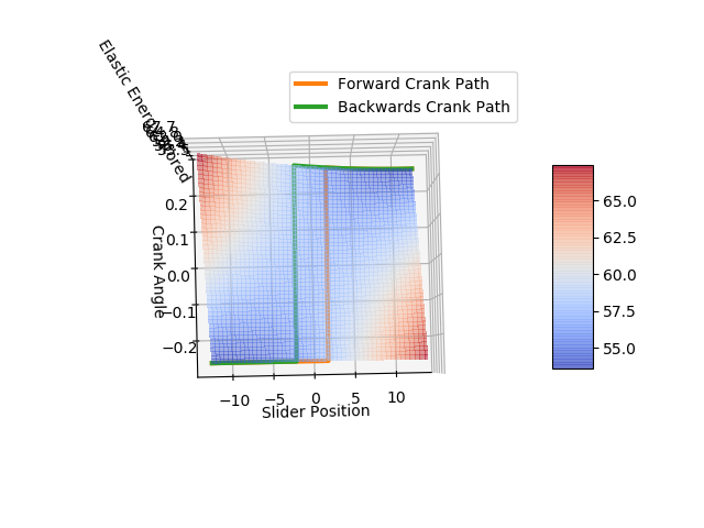 |
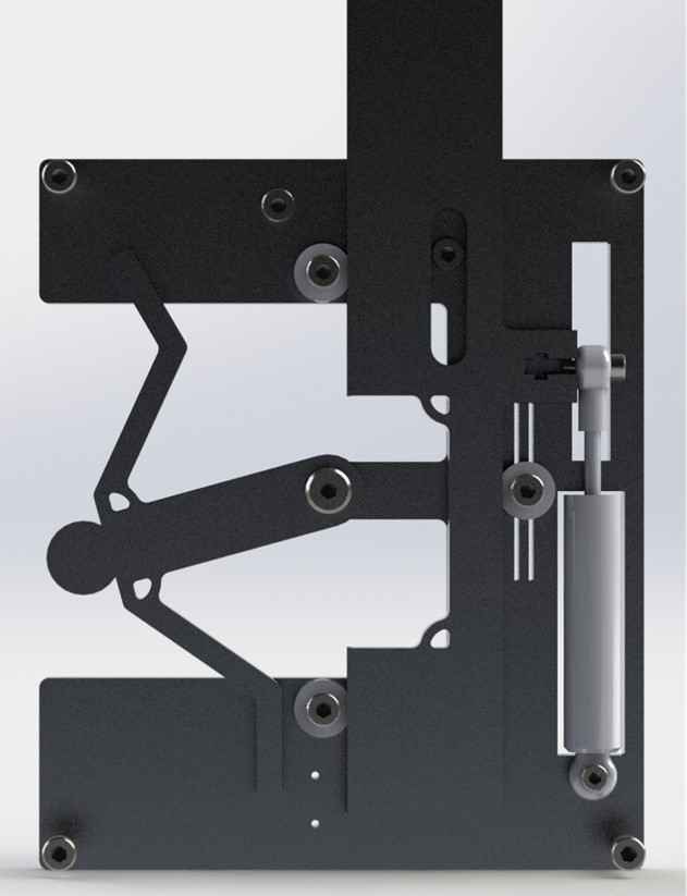
Mathematically, it seems to work, so we set out to design it. Here is a sketch of our intial design alongside with the final CAD
 |
 |
Here’s a GIF of our device working.
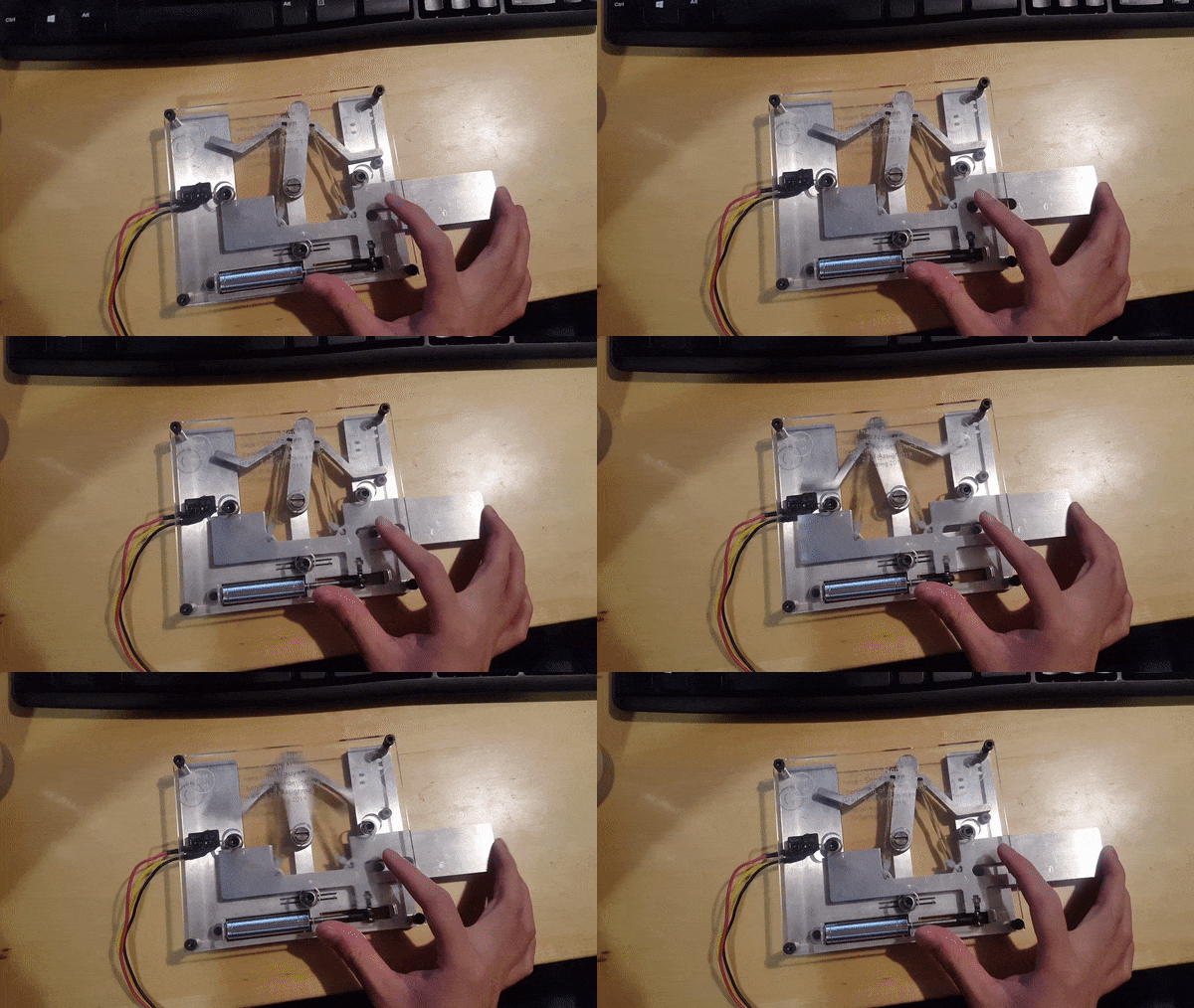
Through our model, we predicted a hysteresis of 4.7 mm, but we ended up seeing a hysteresis of 5.6 mm.
FPGA 3: Abbe’S Principle; Accuracy, Repeatability, Resolution; Sensitive Directions & Reference Features
Flexures Put in Ghastly Applications
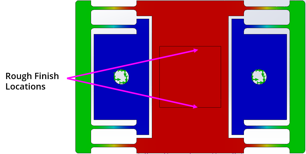
We wanted to do something that will demonstrate sensitive direction on a flexure. So, for this FPGA, we waterjet a flexure and then machined pockets on the flexure. This is normally a terrible idea, but for science, let’s break some end mill.
The setup for our FPGA is like this
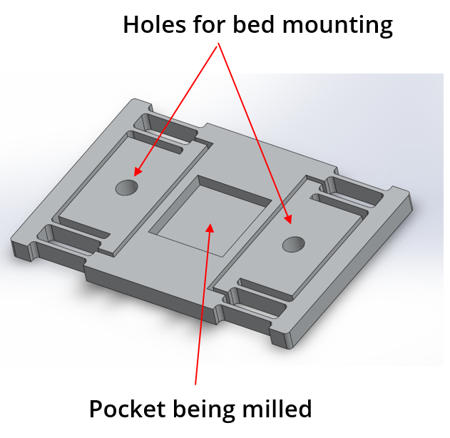
Let’s calculate the stiffness of this flexure in the two directions. This done using FEA in SolidWorks.
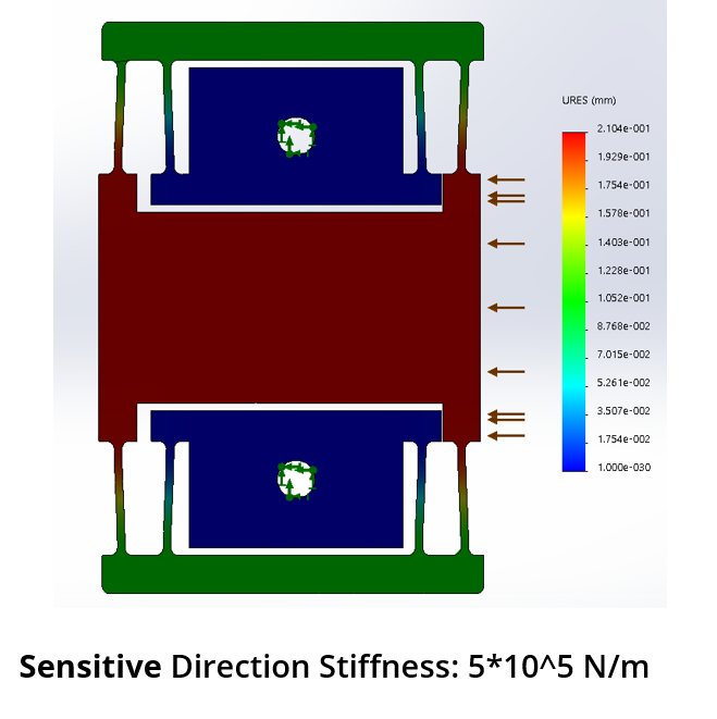 |
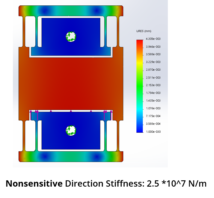 |
Next, let’s figure out the cutting forces involved in pocketing out a hole. Using the machinery handbook, a spreadsheet is created to calculated the forces. Thank you to Julian Leland from Swartmroe College for providing the initial template for this spreadsheet.
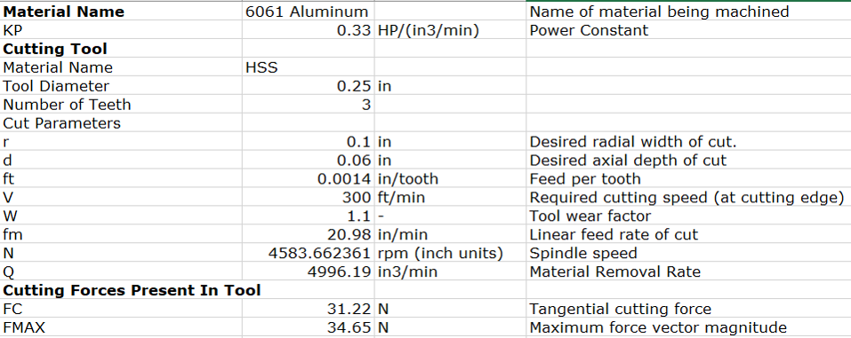
Using this we predict a variation of 0.08 mm on the finished in one surface of the pocket and not on the other.
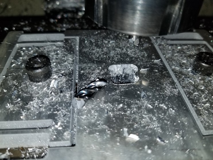
It actually took a lot of work to get this shitty setup to work on the CNC machine. There was so much vibration from the work piece that we basically either started friction welding or just breaking end mills. In the end, a lot of finickying around with the settings and many many flood coolant got us some result.
 |
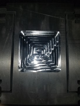 |
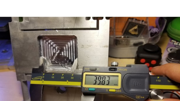
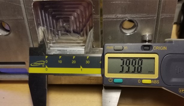
The result is pretty close to what we expected. The deflection along the sensitie axis resulted in each corresponding face being shrunk by 0.075 mm compared to our 0.08 mm prediction. On the other hand, the other axis is not as affected. The pocketed hole supposed to have a dimension of 40x40 mm.
 |
 |
FPGA 4: Centers of Action, Symmetry, Reciprocity
Freaky Pulleys Going Axially
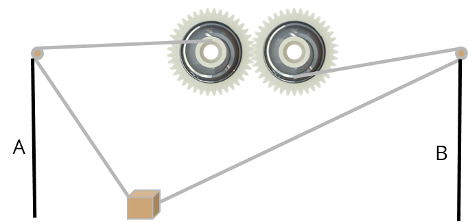
In this FPGA, we wanted to design something to demonstrate reciprocity. The idea is to create a straight virtue rail using strings and two pulleys. This is pretty hard to explain in words, so let’s look at diagram of it first.
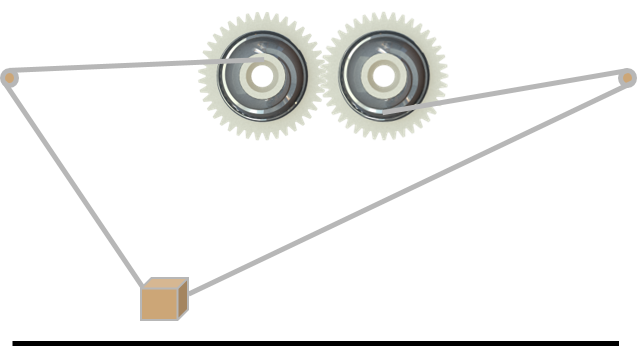
The two pulleys have string wound up in it, and at its end, a mass is attached. The rate at which the pulley take in or release string is carefully calculated such that the attached mass will only move horizontally. The math is just some basic differential equations. Th
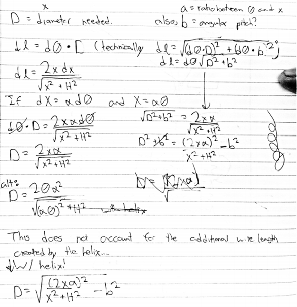
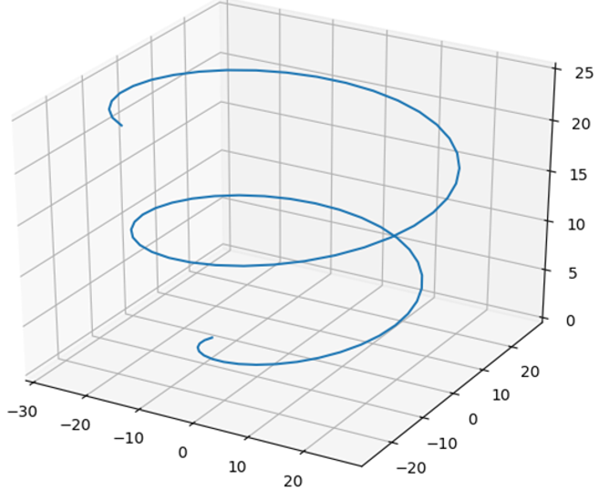
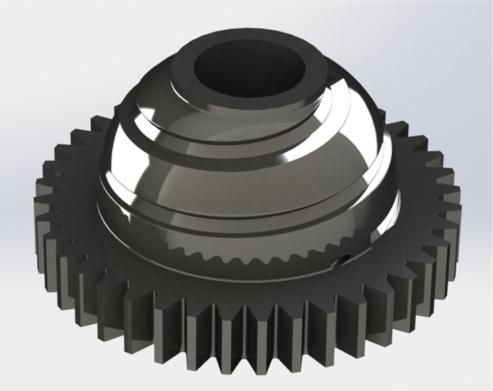
Then we used a python script to generate the basic shape of the pulley. The script generate a path of the continuously changing pulley’s radius. This path is exported to a file and then used by SolidWorks to CAD the pulley.
(click to see code)
import numpy as np
import matplotlib.pyplot as plt
from mpl_toolkits.mplot3d import Axes3D

# input parameters
a = 15  # ratio of pulley angle (radians) to x distance traveled (mm)
H = 100  # distance between pulley and object (mm)
W = 300  # distance between pulleys (mm)
x_padding = 50  # padding between x travel and pulley spacing (mm)
pulley_height = 25  # width of pulley (mm)

# resolution
num_points = 75
# derived figures
x_min = x_padding
x_max = W - x_padding

xs = np.linspace(x_min, x_max, num_points)
thetas = xs / a
pitch = pulley_height / (thetas[-1] - thetas[0])

ds = np.sqrt(np.square(2 * xs * a) / (np.square(xs) + np.square(H)) - np.square(pitch))

# exporting to solidworks curve format

p_x_left = np.cos(thetas) * ds
p_x_right = -np.cos(thetas) * ds
p_y_left = np.sin(thetas) * ds
p_y_right = np.sin(thetas) * ds
p_z_left = np.linspace(0, pulley_height, num_points)
p_z_right = np.linspace(pulley_height, 0, num_points)


# previewing helix shape
fig = plt.figure()
ax = fig.gca(projection='3d')
ax.plot(p_x_left, p_y_left, p_z_left, label='left_pulley')
# ax.plot(p_x_right, p_y_right, p_z_right, label='right_pulley')
ax.legend()

plt.show()


# saving path to file
with open('output_left.sldcrv', 'w') as file:
    output = '\n'.join(' '.join((str(x), str(y), str(z)))
                       for x, y, z in np.vstack((p_x_left, p_y_left, p_z_left)).T)
    file.write(output)

with open('output_right.sldcrv', 'w') as file:
    output = '\n'.join(' '.join((str(x), str(y), str(z)))
                       for x, y, z in np.vstack((p_x_right, p_y_right, p_z_right)).T)
    file.write(output)
 |
 |
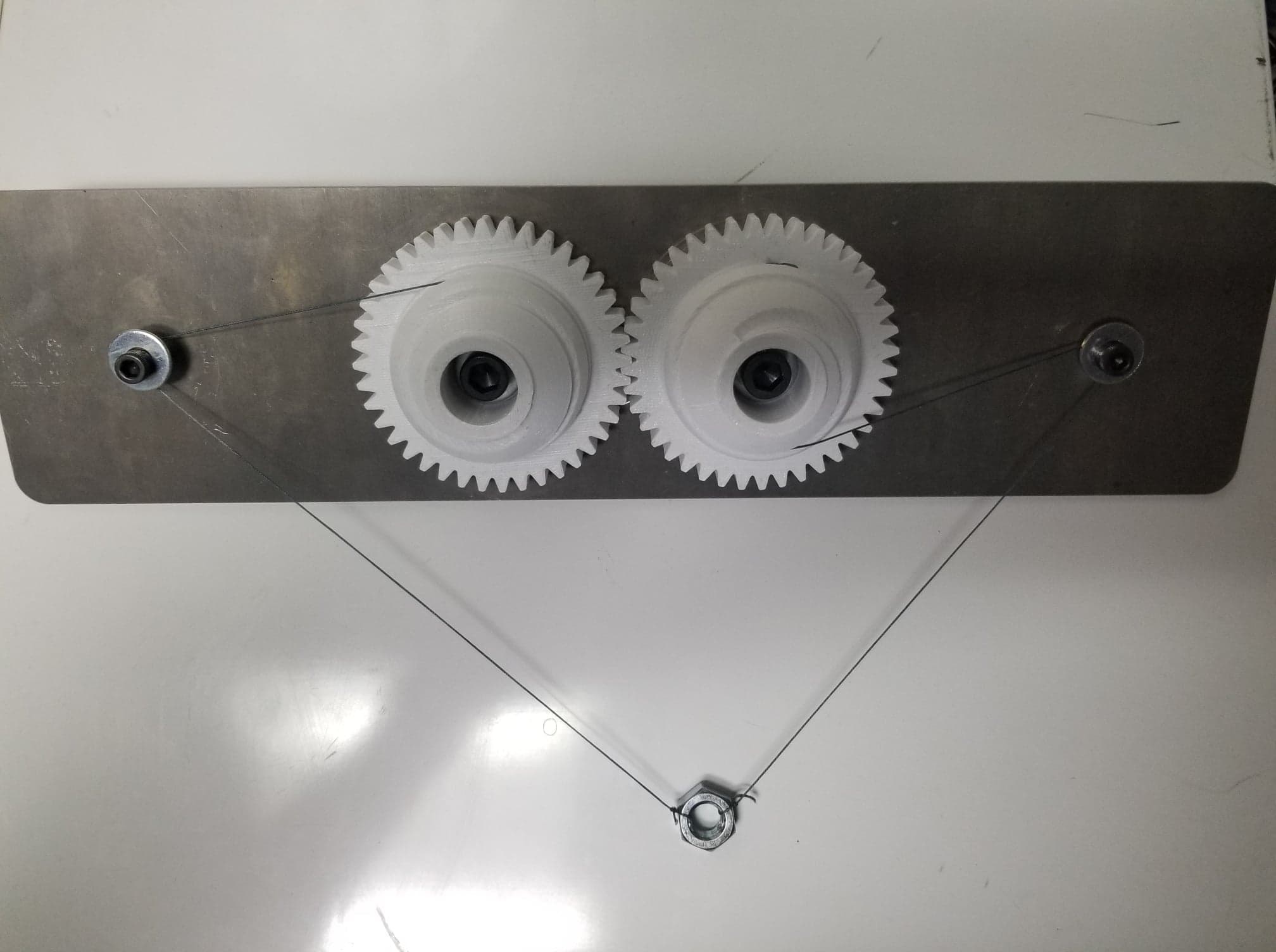
The device then is mounted on an aluminum plate.
Here’s a GIF of the device working.
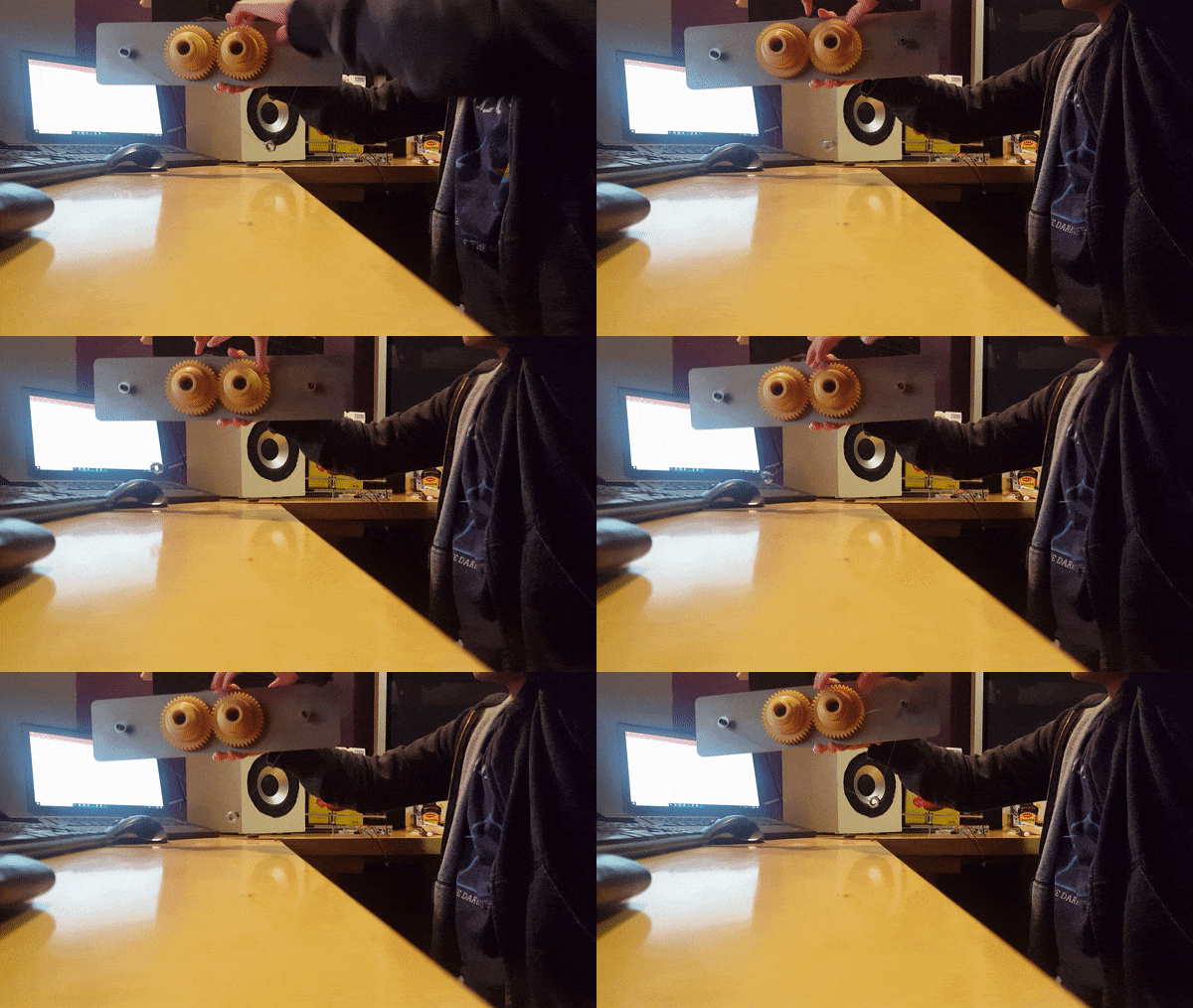
We expected the device to move in a straight line, but out of the three prototypes we built, none of them could move perfectly in a straight line. This is probably due to that fact that the device is extremely sensitive to initial condiction. The mass must be attached at exactly the right length of string with the respect to each of the two pulleys. This is really hard to do manually by hand. A better method must be developed to this last step. Additionally, more second order effects must be considered to get a better straight line.
 |
 |
FPGA 5: Parallel Axis Theorem, Structural Loops
Figure Pulling Great mAss
Do you know about the phenomenom where a spinning ice skater will pull their arms inward to spin even faster? We essentially wanted to make a device that does this to demonstrate Parallel Axis Theorem. The FPGA is a flywheel that has a changing moment of inertia (think mechanical tetherball). A sketch of the final concept can be seen below.

To mathematically analyse this system, we derived an equation of motion using Legrangian Mechanics. This method works by writing the equation of energy of the system and taking derivative. Simple enough…….. Actually, it’s not simple at all. The model works to conserve energy well enough, but as you add a generalized force to change the moment of inertia of the system. I get infinite energy. Additionally, I didn’t have quite enough time to add in non-conservative forces (friction) to the model. The math here just shows that the concept works, but it doesn’t actually do that good of a job describing the device. I will try to redo this if I have more time.
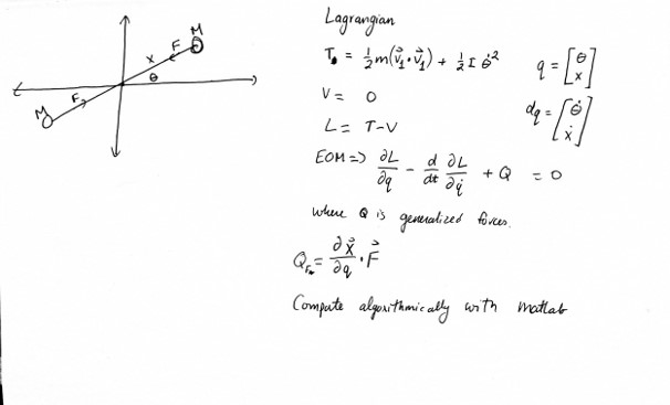
Below is the code I wrote in Matlab to derive the equation of motion and do a dynamic simulation with ODE45.
Deriving the equations of motion with Lagrangian. (Excuse my poor naming convention. I got lazy and reused a previously made code.)
(click to see code)
clear
name = 'leg';

% Define variables for time, generalized coordinates + derivatives, controls, and parameters
syms t th1 dth1 x dx real
syms m1 real
syms l_OA l_OB l_AC l_DE real
syms tau1 tau2 Fx Fy real

% Group them
q   = [th1  ; th2 ];        % generalized coordinates
dq  = [dth1 ; dth2];        % first time derivatives
ddq = [ddth1;ddth2];        % second time derivatives
u   = [tau1 ; tau2];        % controls
F   = [Fx ; Fy];

p   = [m]';        % parameters

% Generate Vectors and Derivativess
ihat = [0; 1; 0];
jhat = [1; 0; 0];
khat = cross(ihat,jhat);

e1hat =  cos(th1)*ihat - sin(th1)*jhat;

ddt = @(r) jacobian(r,[q;dq])*[dq;ddq]; % a handy anonymous function for taking time derivatives


rA = l_OA * e1hat;

r_m1 = l_OA * e1hat;
r_m2 = l_OA * -e1hat;

dr_m1 = ddt(r_m1);
dr_m2 = ddt(r_m2);

% Calculate Kinetic Energy, Potential Energy, and Generalized Forces
F2Q = @(F,r) simplify(jacobian(r,q)'*(F));    % force contributions to generalized forces
M2Q = @(M,w) simplify(jacobian(w,dq)'*(M));   % moment contributions to generalized forces


omega1 = dth1;
omega2 = dth1 + dth2;
omega3 = dth1 + dth2;
omega4 = dth1;

T1 = (1/2)*m1 * dot(dr_m1,dr_m1) + (1/2) * I1 * omega1^2;
T2 = (1/2)*m2 * dot(dr_m2,dr_m2) + (1/2) * I2 * omega2^2;
T3 = (1/2)*m3 * dot(dr_m3,dr_m3) + (1/2) * I3 * omega3^2;
T4 = (1/2)*m4 * dot(dr_m4,dr_m4) + (1/2) * I4 * omega4^2;

Vg1 = m1*g*dot(r_m1, -ihat);
Vg2 = m2*g*dot(r_m2, -ihat);
Vg3 = m3*g*dot(r_m3, -ihat);
Vg4 = m4*g*dot(r_m4, -ihat);

T = simplify(T1 + T2 + T3 + T4);
Vg = Vg1 + Vg2 + Vg3 + Vg4;
Q_tau1 = M2Q(tau1*khat,omega1*khat);
Q_tau2 = M2Q(tau2*khat,omega2*khat);
Q_tau2R= M2Q(-tau2*khat,omega1*khat);


Q_tau = Q_tau1+Q_tau2 + Q_tau2R;

Q = Q_tau;

% Assemble the array of cartesian coordinates of the key points
keypoints = [rA(1:2) rB(1:2) rC(1:2) rD(1:2) rE(1:2)];

%% All the work is done!  Just turn the crank...
% Derive Energy Function and Equations of Motion
E = T+Vg;
L = T-Vg;
eom = ddt(jacobian(L,dq).') - jacobian(L,q).' - Q;


% Rearrange Equations of Motion
A = jacobian(eom,ddq);
b = A*ddq - eom;

% Equations of motion are
% eom = A *ddq + (coriolis term) + (gravitational term) - Q = 0
Mass_Joint_Sp = A;
Grav_Joint_Sp = simplify(jacobian(Vg, q)');
Corr_Joint_Sp = simplify( eom + Q - Grav_Joint_Sp - A*ddq);

% Compute foot jacobian
J = jacobian(rE,q);

% Compute ddt( J )
dJ= reshape( ddt(J(:)) , size(J) );

% Write Energy Function and Equations of Motion
z  = [q ; dq];

rE = rE(1:2);
drE= drE(1:2);
J  = J(1:2,1:2);
dJ = dJ(1:2,1:2);

matlabFunction(A,'file',['A_' name],'vars',{z p});
matlabFunction(b,'file',['b_' name],'vars',{z u p});
matlabFunction(E,'file',['energy_' name],'vars',{z p});
matlabFunction(rE,'file',['position_foot'],'vars',{z p});
matlabFunction(drE,'file',['velocity_foot'],'vars',{z p});
matlabFunction(J ,'file',['jacobian_foot'],'vars',{z p});
matlabFunction(dJ ,'file',['jacobian_dot_foot'],'vars',{z p});

matlabFunction(Grav_Joint_Sp ,'file', ['Grav_leg'] ,'vars',{z p});
matlabFunction(Corr_Joint_Sp ,'file', ['Corr_leg']     ,'vars',{z p});
matlabFunction(keypoints,'file',['keypoints_' name],'vars',{z p});
Dynamic Simulation with ODE45.
(click to see code)
function simulate_leg()

    %% Definte fixed paramters (obtained from CAD)
    m1 =.02 + .210;         m2 =.0225;
    m3 = .004;              m4 = .017;
    I1 = 45.389 * 10^-6;    I2 = 22.918 * 10^-6;
    I3 = 3.2570 * 10^-6;    I4 = 22.176 * 10^-6;
    l_OA=.011;              l_OB=.042;
    l_AC=.096;              l_DE=.096;
    l_O_m1=0.0364;          l_B_m2=0.040;
    l_A_m3=1/2 * l_AC;      l_C_m4=1/2 * (l_DE+ l_OB-l_OA);
    g = 9.81;

    %% Parameter vector
    p   = [m1 m2 m3 m4 I1 I2 I3 I4 l_O_m1 l_B_m2 l_A_m3 l_C_m4 l_OA l_OB l_AC l_DE g]';

    %% Perform Dynamic simulation
    tspan = [0 2];
    z0 = [-pi/4; pi/2; 0; 0];
    opts = odeset('AbsTol',1e-8,'RelTol',1e-6);
    sol = ode45(@dynamics,tspan,z0,opts,p);

    %% Compute Energy
    E = energy_leg(sol.y,p);
    figure(1); clf
    plot(sol.x,E);xlabel('Time (s)'); ylabel('Energy (J)');

    %% Compute foot position over time
    rE = zeros(2,length(sol.x));
    for i = 1:length(sol.x)
        rE(:,i) = position_foot(sol.y(:,i),p);
    end

    w =100;
    % Plot desired and actuatl foot trajectories
    figure(2); clf;
    plot(sol.x,rE(1,:),'r','LineWidth',2)
    hold on
    plot(sol.x,0.025 * cos(w*sol.x) ,'r--');
    plot(sol.x,rE(2,:),'b','LineWidth',2)
    plot(sol.x,-.125+0.025*sin(w*sol.x) ,'b--');

    xlabel('Time (s)'); ylabel('Position (m)'); legend({'x','x_d','y','y_d'});

    %% Animate Solution
    figure(3); clf;
    hold on

    %% Optional, plot foot target information
    % Target traj. Q 1.6
    plot( .025*cos(0:.01:2*pi), -.125+.025*sin(0:.01:2*pi),'k--');

    animateSol(sol,p);
end

function tau = control_law(t,z,p)
    % Controller gains, Update as necessary for Problem 1
    K_x = 40; % Spring stiffness X
    K_y = 40; % Spring stiffness Y
    D_x = 4;  % Damping X
    D_y = 4;  % Damping Y

    % Desired position of foot is a circle
    w   = 30;
    rEd = [0 -.125 0]' + .025*[cos(w*t) sin(w*t) 0]'; % Desired position of foot
    vEd = .025*[-sin(w*t)*w cos(w*t)*w 0]'; % Desired velocity of foot

    rE = position_foot(z,p);
    vE = velocity_foot(z,p);
    J  = jacobian_foot(z,p);

    % Compute virtual foce
    f  = [K_x * (rEd(1) - rE(1) ) - D_x * (vE(1) - vEd(1) ) ;
          K_y * (rEd(2) - rE(2) ) - D_y * (vE(2) - vEd(2) ) ];

    % Map to joint torques
    tau = J' * f;
end

function tau = control_law_extended(t,z,p)
 % Controller gains, Update as necessary for Problem 1
    K_x = 40; % Spring stiffness X
    K_y = 40; % Spring stiffness Y
    D_x = 4;  % Damping X
    D_y = 4;  % Damping Y

    % Desired position of foot is a circle
    w   = 100;
    rEd = [0 -.125 0]' + .025*[cos(w*t) sin(w*t) 0]'; % Desired position of foot
    vEd = .025*[-sin(w*t)*w cos(w*t)*w 0]'; % Desired velocity of foot
    aEd = [-.025*w^2*cos(t*w) -.025*w^2*sin(w*t)]';

    rE = position_foot(z,p);
    vE = velocity_foot(z,p);
    J  = jacobian_foot(z,p);
    dJ = jacobian_dot_foot(z,p);

    %Compute dynamic coefficients
    M = A_leg(z,p);
    lambda = inv(J')*M*inv(J);
    V = Corr_leg(z,p);
    mu = inv(J')*V-lambda*dJ*z(3:4);
    G = Grav_leg(z,p);
    rho = inv(J')*G;


    % Compute virtual foce
    f  = [K_x * (rEd(1) - rE(1) ) - D_x * (vE(1) - vEd(1) ) ;
          K_y * (rEd(2) - rE(2) ) - D_y * (vE(2) - vEd(2) ) ];

    f_new = f + lambda*aEd + rho;
    % Map to joint torques
    tau = J' * f_new;
end


function dz = dynamics(t,z,p)
    % Get mass matrix
    A = A_leg(z,p);

    % Compute Controls
    tau = control_law_extended(t,z,p);

    % Get b = Q - V(q,qd) - G(q)
    b = b_leg(z,tau,p);

    % Solve for qdd.
    qdd = A\b;
    dz = 0*z;

    % Form dz
    dz(1:2) = z(3:4);
    dz(3:4) = qdd;
end

function animateSol(sol,p)
    % Prepare plot handles
    hold on
    h_OB = plot([0],[0],'LineWidth',2);
    h_AC = plot([0],[0],'LineWidth',2);
    h_BD = plot([0],[0],'LineWidth',2);
    h_CE = plot([0],[0],'LineWidth',2);


    xlabel('x'); ylabel('y');
    h_title = title('t=0.0s');

    axis equal
    axis([-.2 .2 -.3 .1]);

    %Step through and update animation
    for t = 0:.01:sol.x(end)
        % interpolate to get state at current time.
        z = interp1(sol.x',sol.y',t)';
        keypoints = keypoints_leg(z,p);

        rA = keypoints(:,1); % Vector to base of cart
        rB = keypoints(:,2);
        rC = keypoints(:,3); % Vector to tip of pendulum
        rD = keypoints(:,4);
        rE = keypoints(:,5);

        set(h_title,'String',  sprintf('t=%.2f',t) ); % update title

        set(h_OB,'XData',[0 rB(1)]);
        set(h_OB,'YData',[0 rB(2)]);

        set(h_AC,'XData',[rA(1) rC(1)]);
        set(h_AC,'YData',[rA(2) rC(2)]);

        set(h_BD,'XData',[rB(1) rD(1)]);
        set(h_BD,'YData',[rB(2) rD(2)]);

        set(h_CE,'XData',[rC(1) rE(1)]);
        set(h_CE,'YData',[rC(2) rE(2)]);

        pause(.01)
    end
end
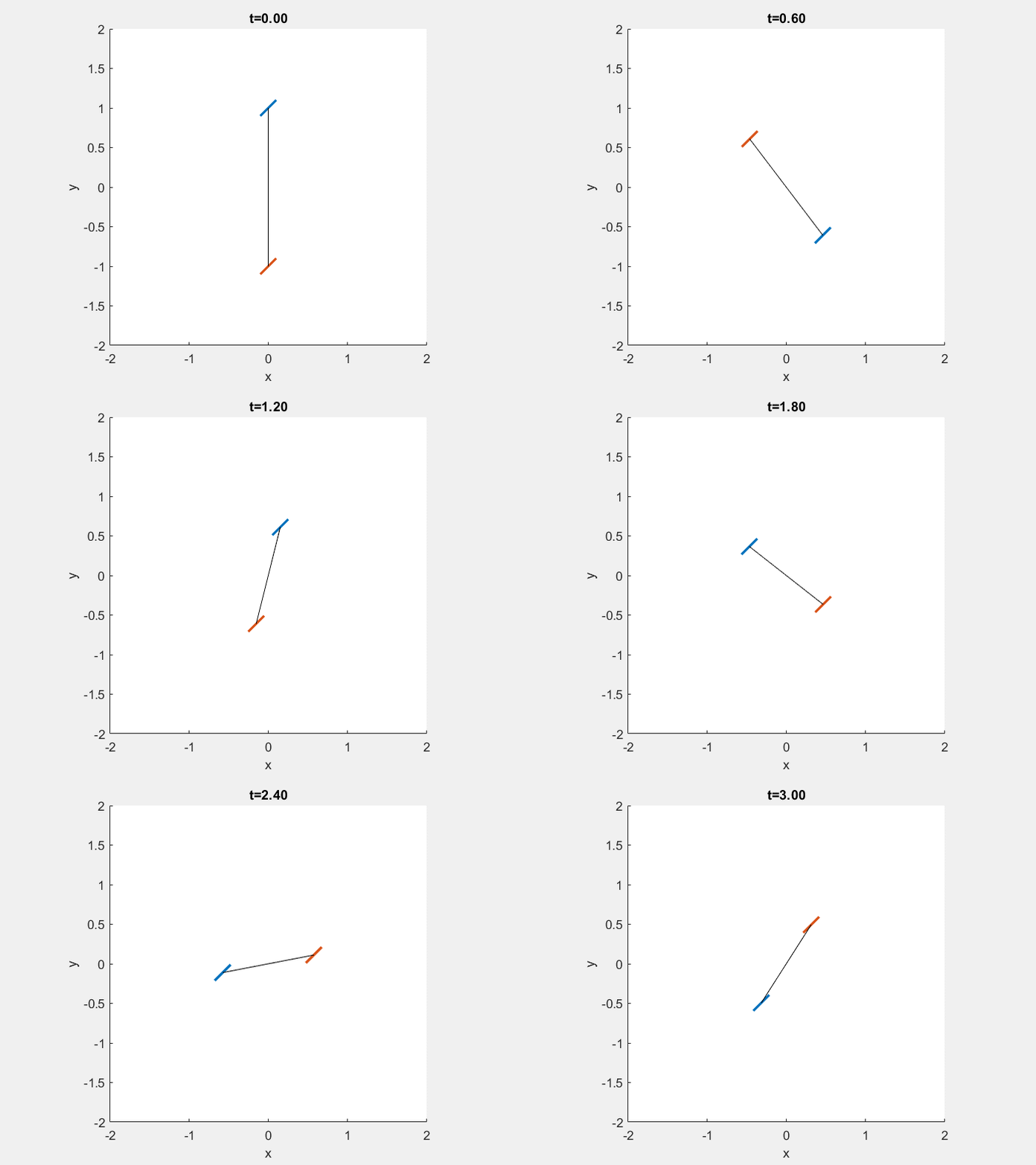
Here’s a GIF of the dynamic simulation.
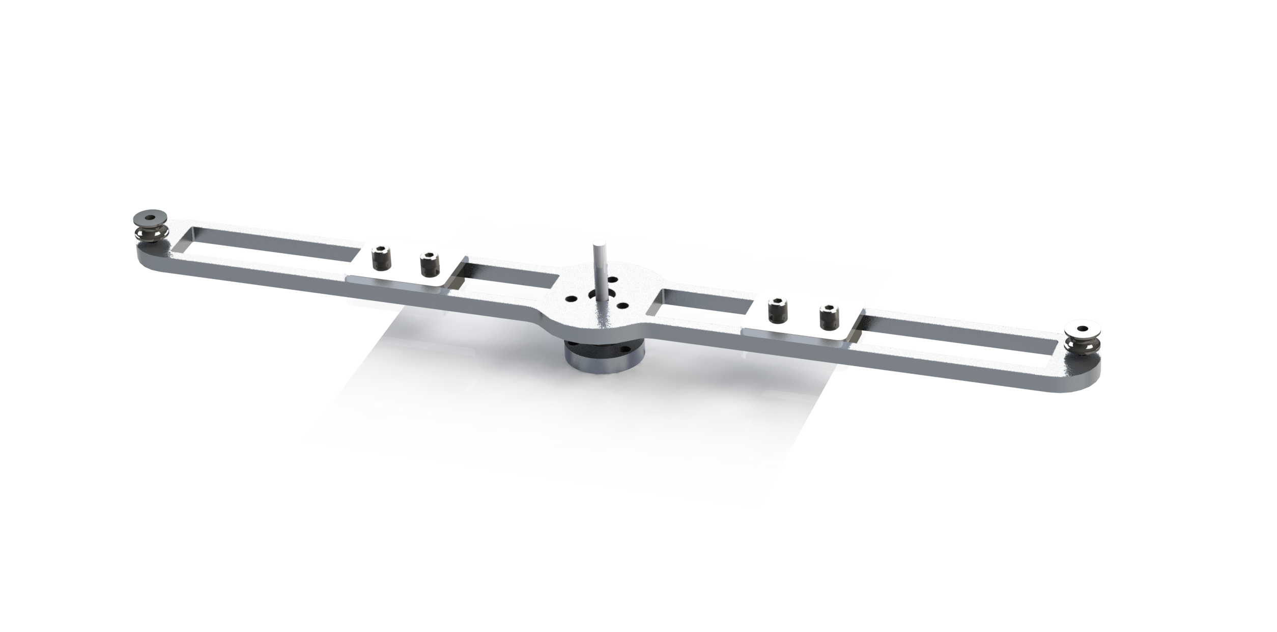
Next, we CAD the device with SolidWorks.
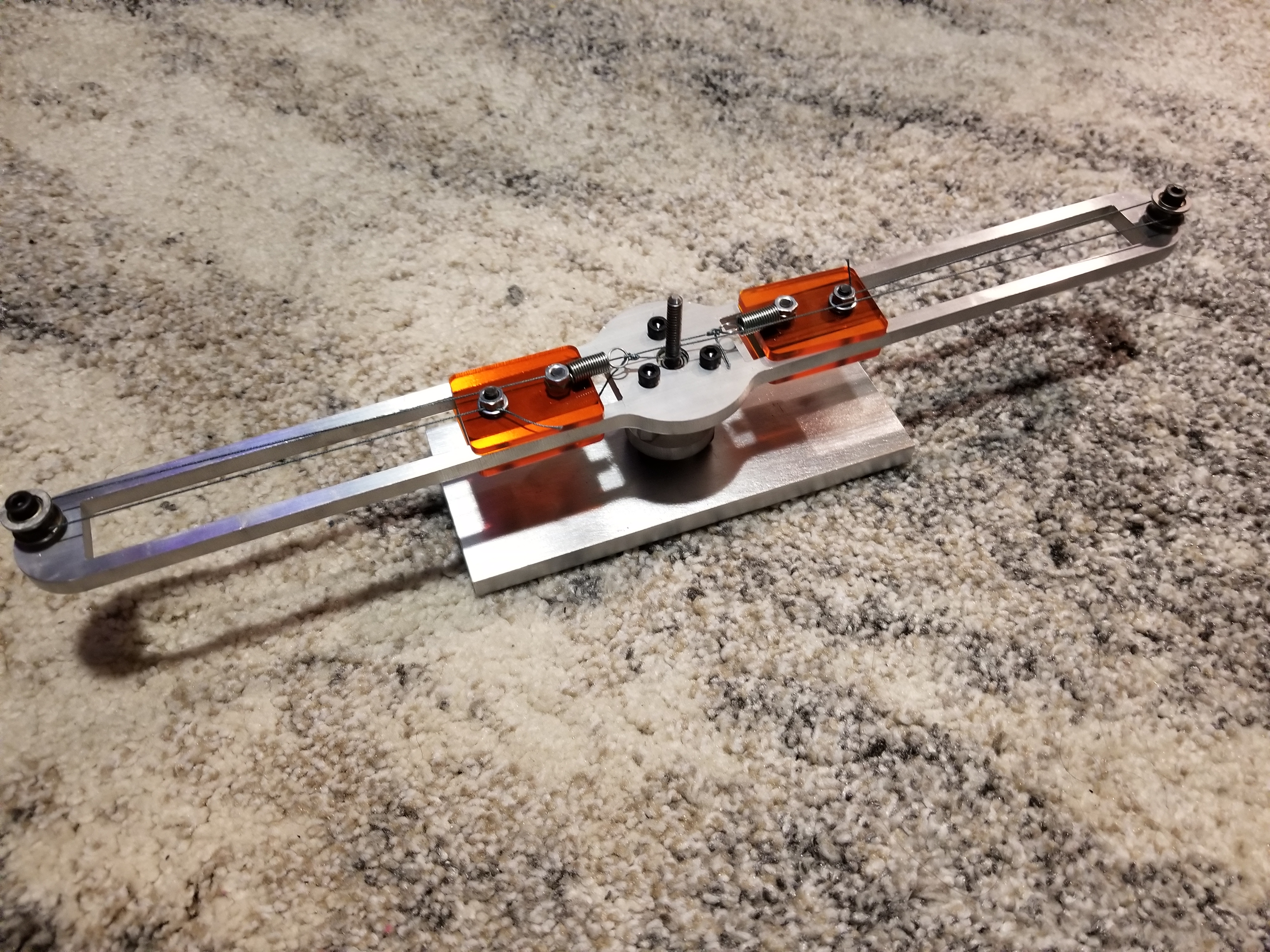
Then we made the thing! It was very simple to make. It’s just a few waterjetted parts. For each device, we only had to pocket 2 holes to fit the bearings. This didn’t take that long at all to make. Here’s a nice photo of the device on my awesome rug.
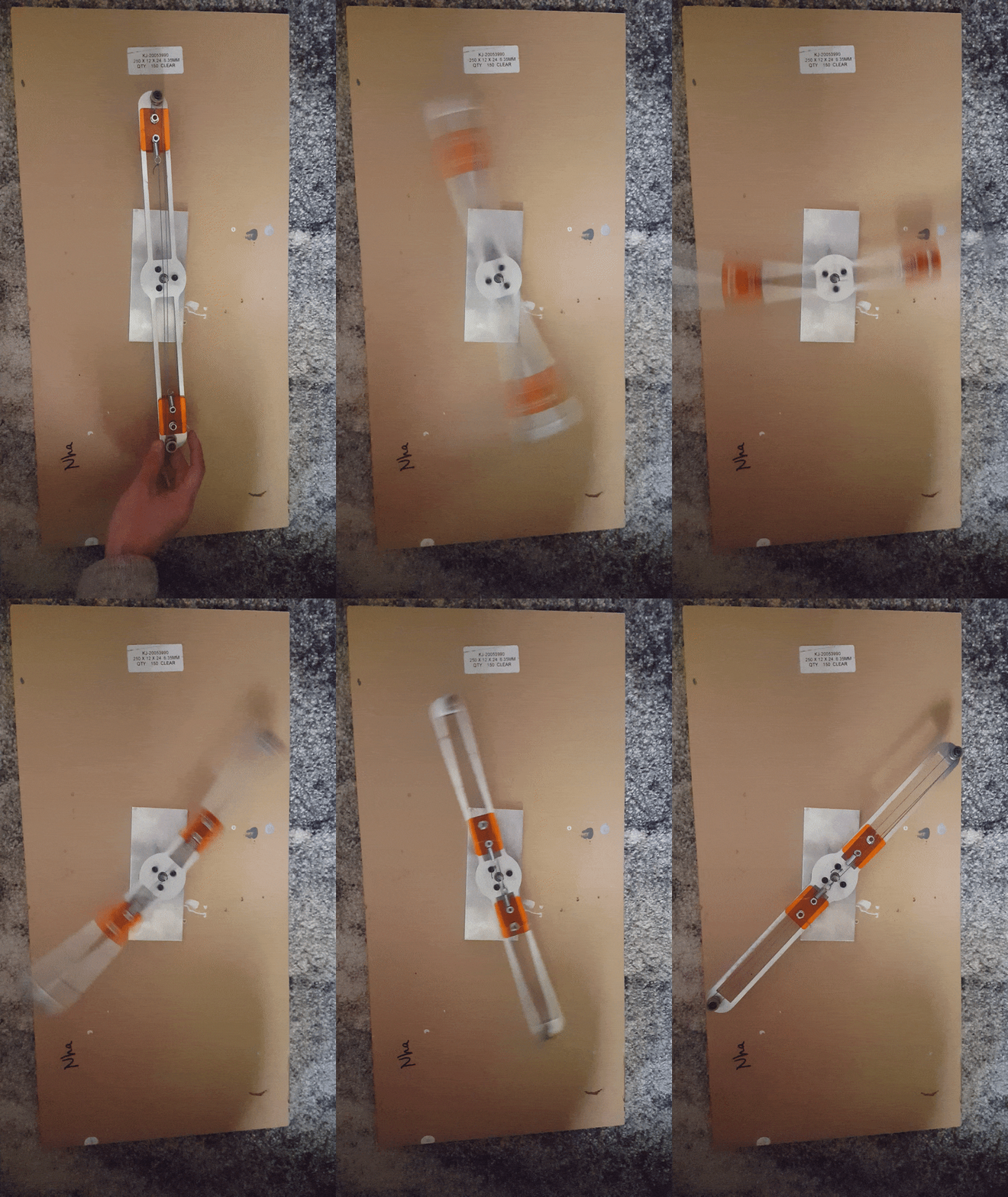
Next, we wanted to actually measure the device if it was actually speeding up or slowing down. Here’s a GIF of the device spinning in both directions.
 |
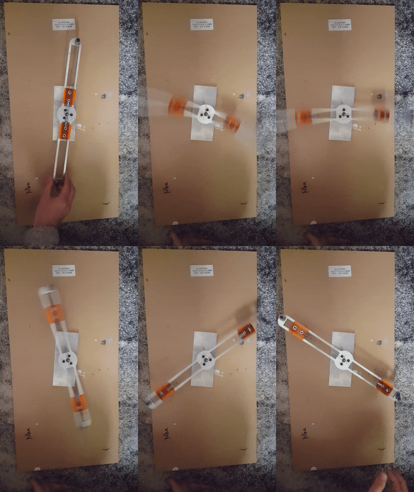 |
The change in angular velocity is so very subtle. We should have going with a way heavier moving mass. Well, that didn’t deter us. Let’s pull out a frame checking softward. I highly recommend using Tracker. It’s super useful to doing frame by frame analysis of a a video. Using this software, we can track the exact movement of the moving mass frame by frame.
Here’s the plot of the collected data. If you stare at it hard enough, you can see that the angular velocity stays roughly constant even with friction when the mass is moving inward. On the other hand, the device spins much slower as the mass is moving outward.
![]()
FPGA 6: Exact Constraint, Elastically Averaged
Friendly Precise Gadget Alignment
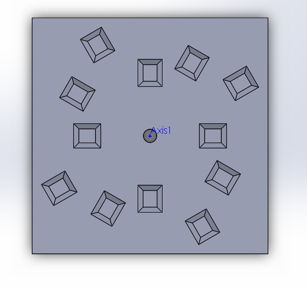
For this FPGA, we built a kinematic coupling to demonstrate the power of exact constraint. A kinematic coupling allows two objects to mate together in the exact same position everytime it taken apart and put together down to nanometer accuracy. It works by constraining the six degrees of freedom that any object has. If you touch an object at the same 6 spots everytime, then the object will orient in the same position everytime. A kinematic coupling does this using 3 balls and 3 v-grooves. For this project, we take this one step further. One one plate, we have 4 orientations on one plate with one orientation every 90 degrees. The v-grooves are offset such that simple rotation can only result in four unique positions.
This diagram below shows the four unique orientations that the 3 v-grooves orient.
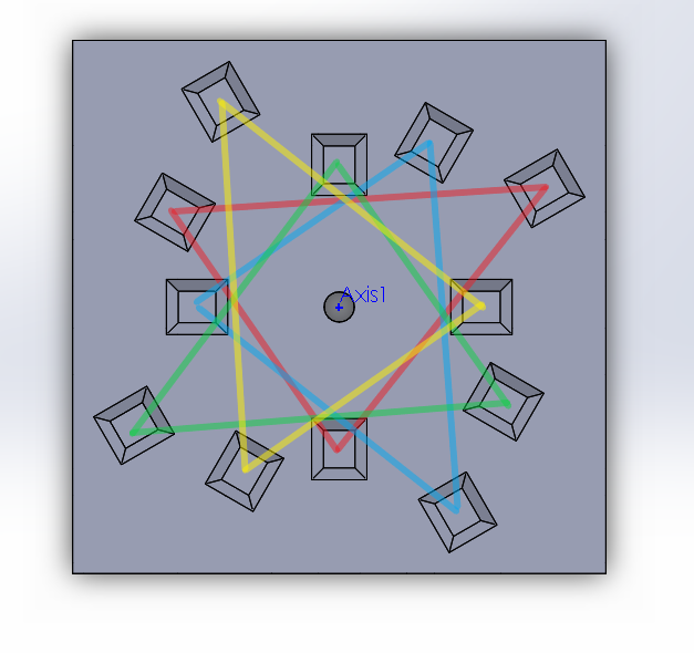
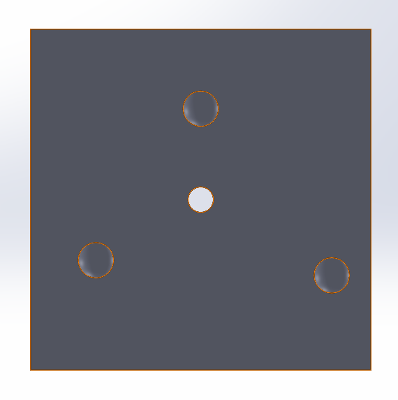
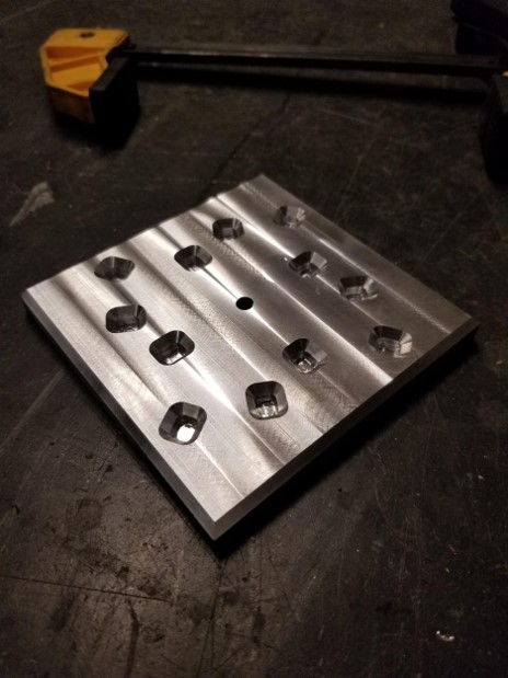
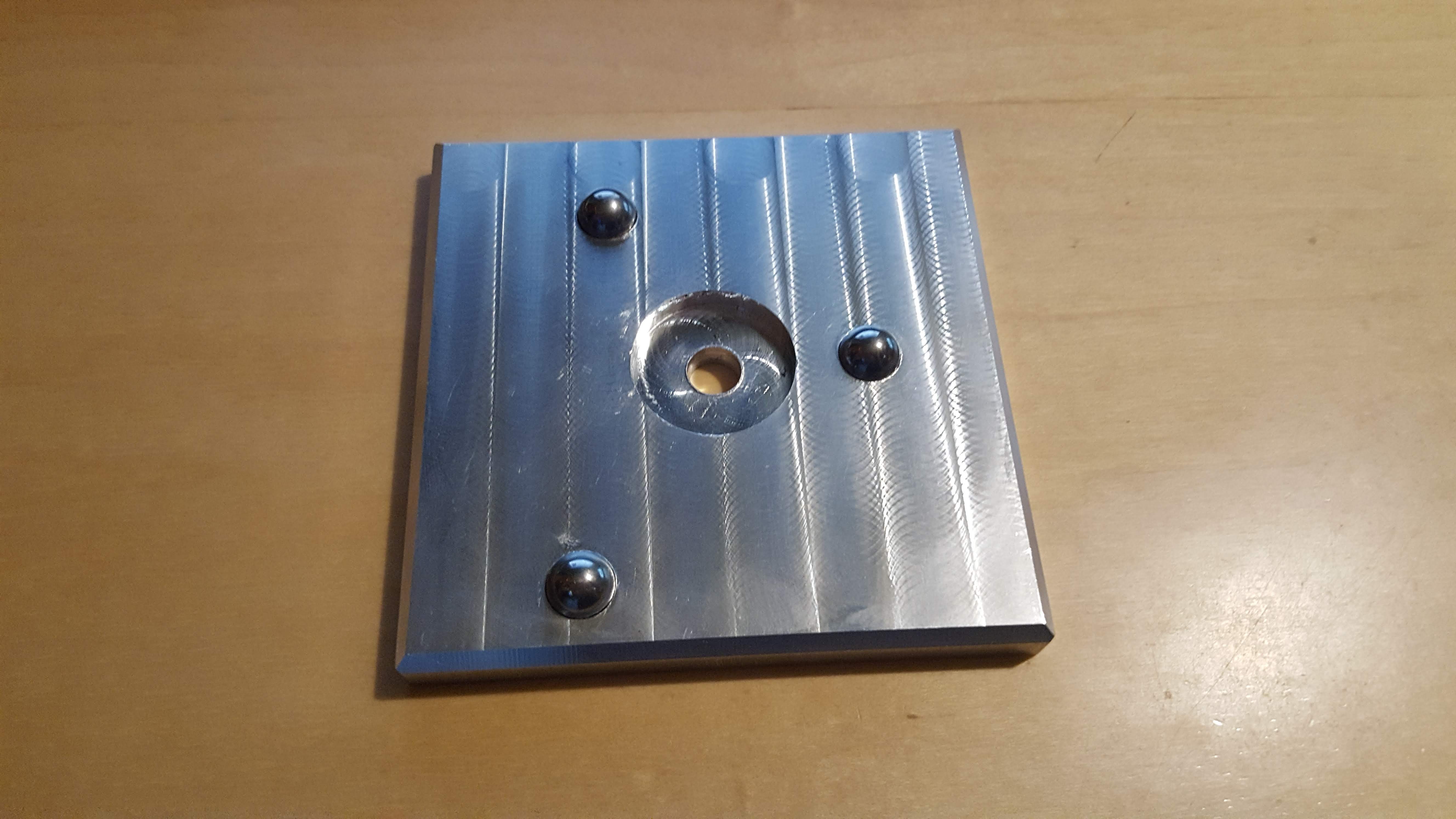
The device is two plates – one with grooves and one with balls.
 |
 |
The device is manufactured using a CNC mill. The balls are press-fit in place.
 |
 |
The analysis for this kinematic coupling relies on using math developed by Professor Slocum at MIT.
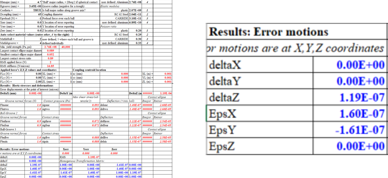
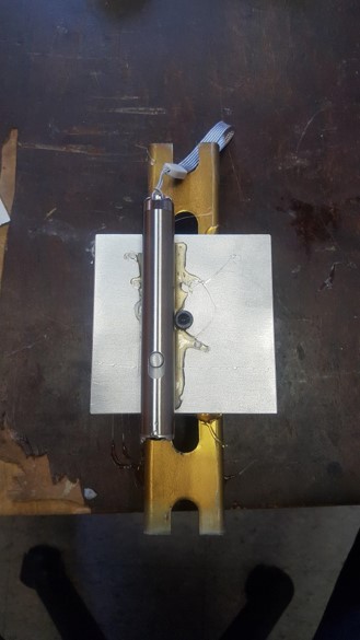
We attempted to measure how good the repeatability of the device, but it was way too good to do. We mounted a laser on the device and shine it to a spot 126 feet away. Then repeatedly uncoupled and coupled the two plates together.
 |
 |
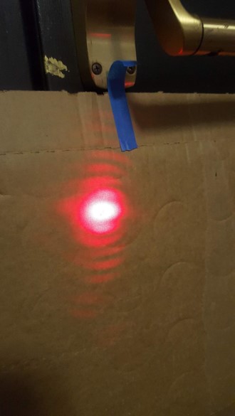 |
After 8 measurements, no difference could be detected with the laser. The beam becomes too scatter to finely determine where it points. We could not measure the repeatability of the device.
